Artificial Intelligence for the Digital Revolution of Pharmaceutical Manufacturing

1. Introduction

Currently, Artificial Intelligence (AI)/Machine Learning (ML) model development programs are scattered and difficult to use, particularly for scientists with less experience in computer programming (e.g., Python). Different computer programs are needed to deploy different AI/ML methods [1-10]. The available AI/ML programs are also not well-suited to integrating with manufacturing processes, limiting their use to model development rather than deployment in real-time applications. Additionally, there are no AI/ML programs dedicated to pharmaceutical manufacturing where achieving consistent product quality is crucial. To widely apply AI/ML in pharmaceutical manufacturing and for regulatory purposes, the emerging AI platform needs to be reliable, simple, user-friendly, and capable of supporting high product quality in real time [11]. 

In this work, the systematic methods and tools needed for continuous pharmaceutical manufacturing processes have been developed. These methods and tools are useful for digitalizing processes, ensuring real-time product quality, digital regulatory evaluation, and addressing other complexities associated with advanced pharmaceutical manufacturing. It will also help expand the understanding of AI-driven next-generation CM processes, address drug shortages, and ensure product quality, thereby enhancing patient safety. The toolbox comprises various ML methods, including Artificial Neural Network (ANN), Dense Neural Network (DNN), Recurrent Neural Networks (RNN), Convolutional Neural Network (CNN), Long Short-Term Memory (LSTM), and Random Forest (RF).

2. Machine Learning (ML) methods

Different ML methods are needed to solve different problems. Some of these ML methods are described in the following sections. 

2.2.1. Artificial Neural Networks (ANN) 

Inspired by the nervous system and chemical-based neuron activation in a biological brain, artificial neural networks are multi-layered black-box approaches to digitally recreating the functionality of non-linear systems using a series of interconnected signals sent to neurons. For example, given a 3-layer fully connected neural network, an array of input values X of size N, an array of output values Y of size N, and hidden layers of size H are shown in Figure 1. The output of X's input values is connected to each node in the hidden layer. Each connection between layers is multiplied by a unique weight wj and summed with a bias b, resulting in equation 1. The output is determined by an activation function that evaluates whether the input exceeds a threshold, as given in equation 2. The Rectifier Linear Unit (ReLu) activation function has been used, which requires less computational power. The training process for all neural networks described in this work follows the ADAM optimizer algorithm [4]. If the number of hidden layers and neurons per layer is significantly higher, the ANN is called a dense neural network (DNN). The dropout parameter can be used in DNN to improve its performance. Dropout is a powerful regularization technique that randomly disables neurons during training to prevent overfitting. For example, a 0.2 dropout rate means that 20% of neurons are turned off during training.

shared property amongst neighboring pixels.

Figure 1: Artificial neural networks (ANN)

2.2.2. Recurrent Neural Networks (RNN)

Artificial Neural Networks (ANNs) and Recurrent Neural Networks (RNNs) differ in structure, function, and application. An RNN has internal memory and can make relatively precise predictions. An RNN is a deep learning model trained to process and convert sequential input data into a specific sequential output. Sequential data is data, such as words, sentences, or time-series data, in which sequential components interrelate according to complex semantic and syntactic rules. An RNN is a software system consisting of many interconnected components that mimic how humans process sequential data, such as translating text from one language to another.

2.2.3. Convolutional Neural Network (CNN)

 A Convolutional Neural Network (CNN) is a type of dense neural network (DNN) most commonly used in computer vision for analysing image and video data [5]. In the context of image processing, a typical DNN would require unraveling the image file from a 2-dimensional (w, h) to a 1-dimensional (1, w*h) format to be correctly fed into the network. However, this data pre-processing would often require

more hidden layers and significantly more processing time due to  each pixel's lacking connected context. For example, classifying shapes such as a drawing of a circle requires on a 160x160 grid requires not only the pixel value but also some shared property amongst neighboring pixels. 

The neighboring pixels' values and the shared property (IE., vector change in pixel value from neighboring pixels) would be lost and may take more hidden layers to process. A series of convolution layers of filters and a pooling layer reduce the input's overall size while still maintaining the image's context. The CNN learns filters that activate when a particular feature is found at certain input coordinates. The filters then get passed to a pooling layer for feature reduction. The pooling layers reduce the image's resolution by combining local neurons' outputs either by global pooling or max pooling. In this case, the pooling Layer is a max-pooling layer, with a maximum kernel size of 60 and 32 filters. The fully connected dense layers are three hidden layers of standard forward ReLU (Rectifier Linear Unit) activation functions.  

Based on a traditional CNN that extracts features from a 2-Dimensional image, the 1D-CNN approach processes an input that spans a time window of arbitrary length, as shown in Figure 2. Unlike the recurring neural network (RNN) approach, the 1D-CNN pre-processes the input data before training and does not require backward propagation. Essentially, the 1D-CNN treats the input time window as a single image of a larger dataset and aims to identify the step response of changing some input with a smaller set of outputs.

2.2.4. Long Short-Term Memory (LSTM) 

Long Short-Term Memory (LSTM) is a form of RNN that uses specialised cells with feedback connections and is used in long sequences of data, such as time-series data in speech and weather forecasting, or text-based image problems [1]. LSTMs have seen implementation in industrial control systems by network package signatures, clustering patient data with time-aware systems, and determining 3D human action recognition [2, 4, 7]. RNNs using an LSTM cell were found to better capture long-term dependencies in datasets due to improved back-propagation, which results in fewer infinite or zero-scaled gradients [3]. Infinite and zero-scaled

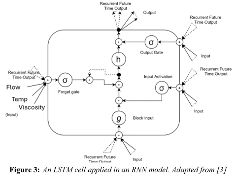
gradients are reduced since both waste memory space and cause errors. An LSTM operates by using segments of the output vector to influence the delta calibration of weights and bias values in each iteration during the training process, and uses previous time steps to determine the adjustments made inside each node's parameter, and are passed to the following forward-backwards layer. The neurons are made with multiple hidden layers of LSTM cells operated with ReLU activation functions [6].

2.2.5. Random Forest (RF)

Random Forests are a machine learning approach that uses an ensemble of randomly generated decision trees to classify or regress by majority vote (see Figure 4). Initially used for classification problems, random forests are effective for regressive multivariate and time-series forecasting problems [9-10]. A decision tree is an intuitive set of binary conditions that branch to a result based on an input's qualities. In the context of a manufacturing process, sensor data inserted into a decision tree passes through simple conditions until the most likely result is decided. Due to the static structure of decision trees, their application for regression analysis with varying input sets is limited. RFs are therefore a better fit due to their flexibility in analysing varying combinations of bootstrapped datasets. Figure 4 provides a simplified visualisation of the random forest process. In this example, an input vector of size 3 (flow rate, temperature, viscosity) is processed by X decision trees to find PX(t), where PX is a series of predicted signal values at time t+tn. The overall best-predicted API concentration values are determined by averaging the probabilistic prediction to determine API concentration at t+tn. For this example, we chose tn = 20. The random forests are trained and analysed in the developed AI/ML toolbox using the sci-kit learn library.

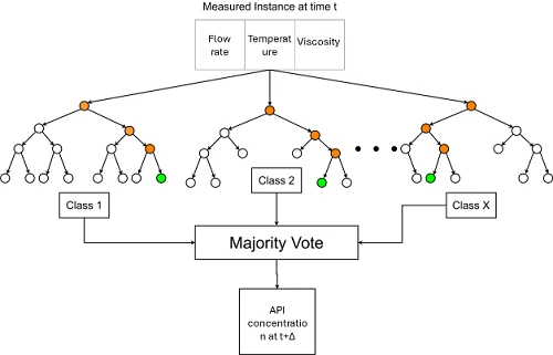
Figure 4: Random Forest structure [9-10]

3. Training, verification, and deployment of the ML models

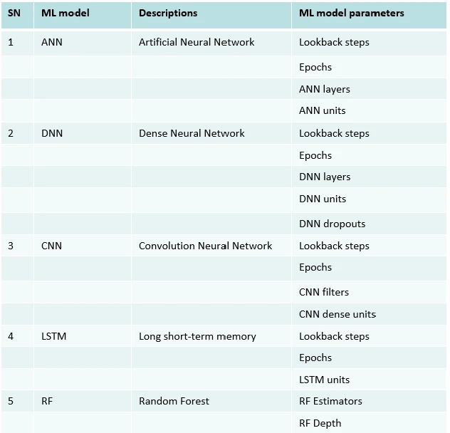
The training and verification of the ML model are complicated tasks; therefore, we proposed a multistep, iterative process. In the first step, the optimal values of the ML parameters need to be identified. The ML parameter example for some of the ML models is listed in Table 1. The second step of the ML model training process involves the identification of the ML model structure and the values of the parameters of each neuron (e.g. weight and bias). The third step is the verification of the ML models using a new data set. For each step, the performance evaluation is based on the statistical parameters. Finally, the ML model can be deployed for its intended applications. All these steps are repeated until the model’s performance is satisfactory.  

Table 1. ML model parameters

4. Conclusions

The different machine learning models, such as ANN, DNN, RNN, CNN, LSTM, and Random Forest (RF), have been investigated. The training, verification, and deployment of ML models are iterative, challenging processes that involve identifying several ML parameters. A systematic methodology has been developed to overcome these challenges. The performance of these machine learning models has been compared for the continuous drug substance manufacturing case study. The current drawbacks of ML approaches include the need for substantial amounts of data to obtain a fully confident model, which requires significant material, resources, and time. To overcome this limitation, a validated flowsheet model or digital twin could be used to train the ML model. 

Acknowledgements

This work is supported by the US Food and Drug Administration (FDA), through grant 75F40125C00089.

References

1. Baytas, I. M., et al. (2017). "Patient Subtyping via Time-Aware Lstm Networks." In Proceedings of the 23rd ACM SIGKDD International Conference on Knowledge Discovery and Data Mining, 65–74.
2. Graves, Alex, Abdel-rahman Mohamed, and Geoffrey Hinton. (2013). "Speech Recognition with Deep Recurrent Neural Networks." In 2013 IEEE International Conference on Acoustics, Speech and Signal Processing, 6645–49. Ieee.
3. Greff, Klaus, Rupesh K Srivastava, Jan Koutnı́k, Bas R Steunebrink, and Jürgen Schmidhuber. (2016). "LSTM: A Search Space Odyssey." IEEE Transactions on Neural Networks and Learning Systems 28 (10): 2222–32.
4. Kingma, D. P., and Ba, J. (2014). "Adam: A Method for Stochastic Optimization." arXiv Preprint arXiv:1412.6980. https://arxiv.org/abs/1412.6980
5. LeCun, et al. (2015). Deep Learning. Nature, 521, 436-444.
6. Nair, Vinod, and Geoffrey E Hinton. (2010). "Rectified Linear Units Improve Restricted Boltzmann Machines." In Icml.
7. Palangi, Hamid, Li Deng, Yelong Shen, Jianfeng Gao, Xiaodong He, Jianshu Chen, Xinying Song, and Rabab Ward. (2016). "Deep Sentence Embedding Using Long Short-Term Memory Networks: Analysis and Application to Information Retrieval." IEEE/ACM Transactions on Audio, Speech, and Language Processing 24 (4): 694–707.
8. O’Connor, T. (2020). FDA Grand Rounds: Modernization of Pharmaceutical Manufacturing through the Adoption of Advanced Technology. https://www.fda.gov/science-research/fda-grand-rounds/fda-grand-rounds-modernization-pharmaceutical-manufacturing-through-adoption-advanced-technology.
9. Qiu, X.,, et al. (2017). "Oblique Random Forest Ensemble via Least Square Estimation for Time Series Forecasting." Information Sciences 420: 249–62.
10. Segal, M., and Yuanyuan X.. (2011). "Multivariate Random Forests." Wiley Interdisciplinary Reviews: Data Mining and Knowledge Discovery 1 (1): 80–87.
11. Singh, R.; Sahay, A.; Muzzio, F.; Ierapetritou, M.; Ramachandran, R. Systematic framework for onsite design and implementation of the control system in continuous tablet manufacturing process. Computers & Chemical Engineering Journal 2014, 66, 186-200.
12. Singh, R., Muzzio, F., Ierapetritou, M., Ramachandran, R. A combined feed-forward/feed-back control system for a QbD based continuous tablet manufacturing process. PROCESSES Journal, 2015, 3, 339-356.